


An intuitive understanding of Bayesian statistics
- May 25, 2020
- 3 min read
In previous post, we mentioned that each locus across genome owns different noise rate due to variety of technical / biological factors. Bayesian method may better detect genuine variants by adding these factors into consideration. Before diving into more sophisticated somatic variant detection method, let’s spend a bit of time on the background of Bayesian inference.
The frame of Bayesian model The main idea of Bayesian statistics is to combine current data with prior experience / data for better estimation. Three major elements in Bayesian model are: Prior probability, Likelihood function and Posterior probability. Assuming we would like to estimate the probability of event y occurring with some prior knowledge θ that is related to y.

Where:
P(θ) is prior probability, representing the probability of event θ.
P(y|θ) is Likelihood function, representing the conditional probability of event y occurring given previous data θ is true.
P(θ|y) is posterior probability, representing the conditional probability of previous data y given current data θ is true.
P(y) is probability of event y occurring
Why combines previous data? Now we like to develop a screening method for cancer that raises in 0.05% of population. In a typical retrospective study, we usually set case-control group (100 patients vs 100 healthy) to develop / evaluate the method. Assuming our method achieves 99% sensitivity and 99% specificity. How good will this method perform in real world screening task?
P(θ) is prior probability, representing the 0.05% occurrence of cancer in population.
P(y|θ) is the probability of being positively screened in patient population, aka sensitivity of 99%
P(y) is the probability of being positively screened in entire population. This includes positively screened patients (0.05%*99%) and positively screened healthy ((1-0.05%)*(1-99%)).
P(θ│y) is posterior probability, representing probability of being a cancer patient in positively screened population, aka positive predictive value (PPV).

Through calculation above, it turns out that only 4.95% positively screened are real cancer patients. This example demonstrates how inappropriate to evaluate the performance of the model when the real world scenario is ignored (in this case, the cancer occurrence in real world population).
An example to demonstrate Bayesian model The essence of Bayesian inference is to combine current data (Likelihood) and previous data (Prior probability) to calculate the Posterior probability. This way we can make better estimation by integrating additional samples or relevant information. We will demonstrate this using an example of estimating the probability of mouse getting cancer. We set a scenario where only limited mouse samples are available in current experiment, we would like to take advantage of data gathered from previous related experiments and use Bayesian method for better estimation.
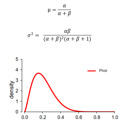
Setting prior probability To model the probability of mouse getting cancer, we use Binomial distribution as Likelihood function where θ is the probability of mouse getting cancer. Beta distribution is used to as Prior probability. We choose Beta distribution because it is a continuous distribution constraint within [0, 1] and can be conveniently seen as probability of probability. Therefore, we have θ~Beta(α,β). When the exact probability of mouse getting cancer is unknown, Beta distribution gives use a rough estimation based on prior knowledge.
Based on previous data, we know the amount of mouse getting cancer and free of cancer (α,β) and can calculate the parameter and shape of Beta distribution (θ~Beta(2.6,9.7),μ=0.211 and σ^2=0.112).
Updating prior probability In currently experiment, we obtained 15 mouse among which five are cancerous. We can now use this additional data to update the parameter of conjugate prior probability and drive posterior distribution.

As demonstrated above, Posterior distribution follows beta(α+k, β+n-k), where k and n-k represents cancerous mouse and healthy mouse in current experiment respectively. The final updated posterior distribution become beta(7.6,19.7) which intuitively is the compromise between Prior and Likelihood as showed in figure above. The final shape of posterior depends on the ‘confidence’ (sample size and variance) we have on prior knowledge and current data.
Comments